Deeplearning techniques have proven to be the most efficient AI tools for computer vision. In this blog post we use a deeplearning convolutional neural network to build a classifier on my baby twins pictures.
When it comes to machine learning practical experiments, the first thing anybody needs are some data. When experimenting for hobby, we often rely on some open and popular dataset such as MNIST or the IMDB reviews. However, it is useful for improving to be confronted with challenges on fresh and unworked data.
Since July 2019 (9-months at the time of the writing), I am the happy father of two lovely twin baby girls: L and J. If I have free private data at scale, it is definitely photos of my kids. Indeed, all our families have been taking pictures of them and, thanks to Whatsapp and other communications means, I have been able to collect a great part of them.
In this post, we will use a state-of-the-art deep learning architecture: Inception ResNetV1 to build a classifier for photo portraits of my girls. We also take benefit of some pretrained weights from facenet dataset. Before that, we will make a detour by tricking a little bit the problem: this will allow us to check our code snippets and review some nice visualization techniques. Then, the InceptionResNetV1 based model will allow us to achieve some interesting accuracy results. We will experiment using Keras backed by Tensorflow. We conducted the computing intensive tasks on a GPU machine hosted on Microsoft Azure.
The code source is available here: on Github. The dataset is obviously composed of personal pictures of my family that I do not want to let openly accessible. In this blog post, the faces of my babies have been intentionally blured to preserve their privacy. Of course, the algorithms whose results are presented here were run with non obfuscated data.
In this post and in the associated source code we reuse some of the models and snippets from the (excellent) book Deep Learning with Python by François Chollet. We also leverage the InceptionResNetv1 implementation from Sefik Ilkin Serengil.
Let us start this post by explaining the problem and why it is not as easy as it may seems to be.
A more complex topic that it seems
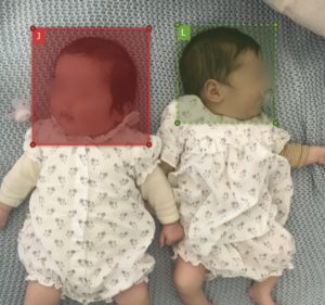
While my baby girls L and J are not identical twins, they definitely are sisters, they do look alike a lot! In addition, the photos were taken since their first days in this world to their 8 months. It is no secret that babies change a lot during their first months. They were born weighing around 2.5 kgs, now they are close to 9 kgs. Even family members whom saw them in their first days have difficult times distinguish them now.
In addition, following their grandmother’s home country tradition L and J were shaved at the age of 4 months. Their haircut is not a way to distinguish them: we have photos before the shaving, during hair regrowth and now with middle to long hairs. Also, many photos were taken with a woolen hat or anything else. Consequently, we will be pushing a little the limits of face recognition.
Our objective in this series of experimentation is to build a photo classifier. Precisely, given a photo we would like to make a 2-class prediction: “Is this photo is the one of L or J?”. We assume then that each picture contains one and only one portrait of one of my two baby girls.
I have collected 1000 raw photos that will be used to create the dataset.
Building the dataset
Photo tagging
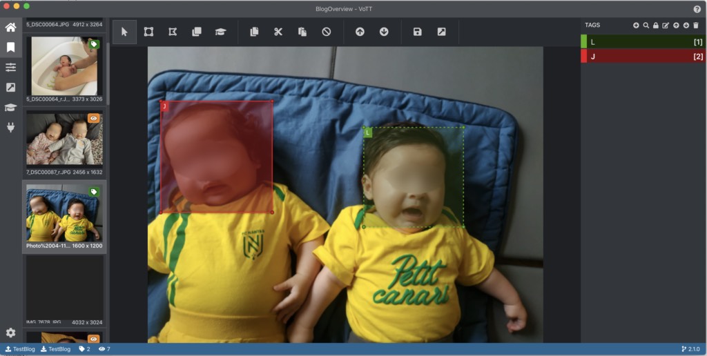
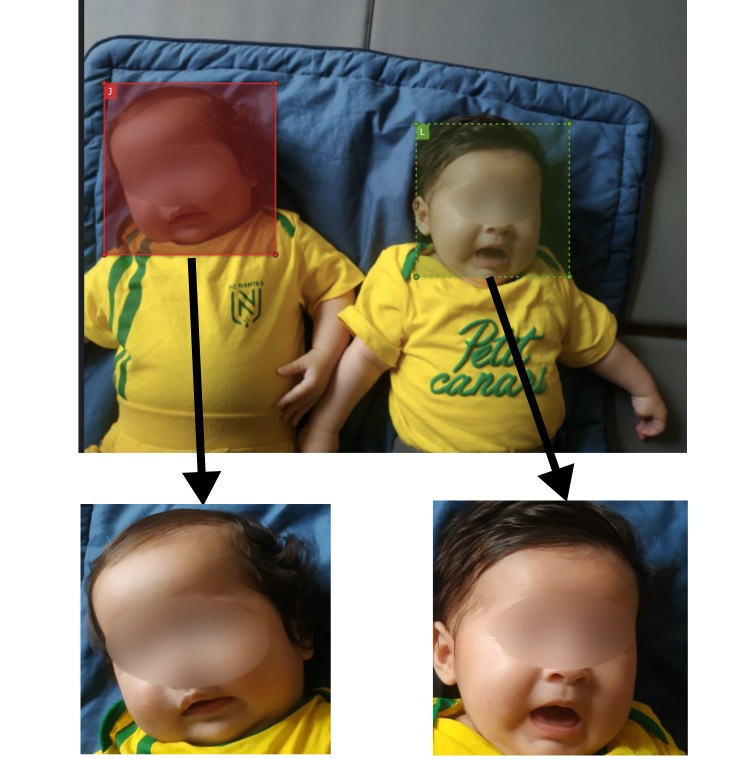
In the raw datasets, some photos contain only L, others only J, some both and some none of them. We exploit these photos to extract face pictures for each girl. To do so, we need to locate precisely the faces in the photos first.
For efficient annotation, I have used an opensource tagging software: VoTT which is supported by Microsoft. The tagging is pretty straightforward and you can quickly annotate the photos with a very intuitive interface. It took me between one and two hours to tag the full dataset.
One of the worries of twins parents, is the fear to favor one child over the other. Well, I am not concerned and data speak for me. Here are the results: after the tagging we have a very well balanced tags repartition with a little more than 600 tags for each of the girls.

Now we will build the picture dataset: where each picture contains the portrait of one of the kid. VoTT provides the tag location within the picture as a JSON format. Therefore, it is easy to crop all files to produce a dataset where each image contains only one kid’s face, see this code snippet.
Splitting the dataset: train, validation, test
As always for any machine learning training procedure, one must separate the original dataset between: 1) training data that will be used to fit the model and 2) validation data that will be used to measure performance of the tuned algorithms. Here we go further by keeping also a third untouched test dataset.
It is always easier to work with an equally balanced dataset. Luckily this is almost the case with the original data. Consequently after processing (mainly shuffling and splitting) we obtain the following repartition in our file system:
The code snippets for splitting and shuffling the dataset is available here.
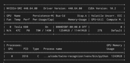
Machine setup - GPU Powered VM
The experiments are conducted with Python 3.6 and Tensorflow GPU 1.15. We use the high level deeplearning library Keras 2.2.4.
We have setup an Ubuntu 18.04 NC6 GPU VM on Microsoft Azure. The NC-series VM use Nvidia Tesla K80 graphic card and Interl Xecon E5-2690 for CPU. With the NC6 version we benefit from 1 GPU and 6 vCPU, this setup maked the following computations perfectly acceptable: all experiments lasted less than few minutes.
This is the second time I do the setup of an Ubuntu machine with Cuda/cudNN and Tensorflow, same as before this was a real pain. The official documentation from Tensorflow is totally incorrect and guides you in the wrong direction. Finally, I managed to have a successful setup with the following Tensorflow-gpu 1.15.0, Keras 2.2.4 and Cuda 10.0 thanks to this StackOverflow post.
For efficient development, I use VSCode with the new SSH Remote extensions which make remote development completely seamless. The experiments are also conducted with IPython Jupyter notebook. And once again VSCode provides out-of-the-shelf SSH tunneling to simplify everything.

First, a simplified problem with tricked data to get started
The experiments provided in this section can be found in this notebook.
Here we will make a small detour by simplifying tricking the challenge. We will add easily detectable geometrical shapes in the images.
Drawing obvious shapes on image classes
When tackling a datascience project, I always think it is great to start really simple. Here, I wanted to make sure that my code snippets were ok so I decided to trick (temporarily) the problem. Indeed, I drawed geometrical shapes on image classes. Precisely, for any J photo, a rectangle is drawn and, for any L photo, an ellipse is inserted. The size, the shape ratio and the filling color are left random. You can see with the two following examples what this looks like:
Of course this completely workarounds and tricks the face recognition problem. Anyway that’s a good starting point to test our setup and code experimentation snippets.
A simple Convnet trained from scratch
For this simplified task we use the basic Convnet architecture introduced by Francois Chollet in his book (see the beginning of the post). Basically, it consists of 4 2D-convolutional layers followed by MaxPooling layers. This constitutes the convolutional base of the model. Then the tensors are flatten and a series of Dense and Dropout layers are added to perform the final classification parts.
97%+ accuracy
Actually this is no surprise that we are able to achieve great classification performance. The algorithms performs without difficulty. To do so we used the standard Data-augmentation techniques. Note that for this task we skipped the rotations.
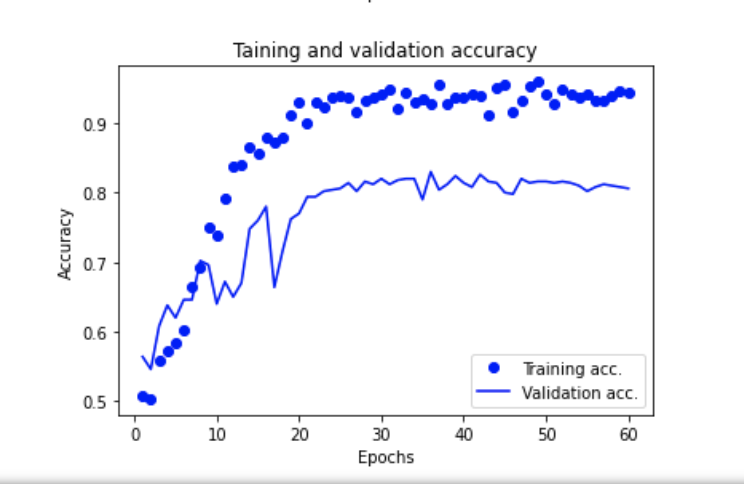
After running the training on 30 epochs we observe the following learning curves.
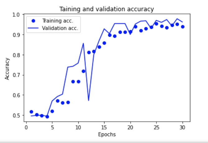
Now that the results seem satisfactory without sign of overfitting (the validation accuracy grows and stalls). It is time to measure performance on the test sets composed of the 200 pictures left aside.
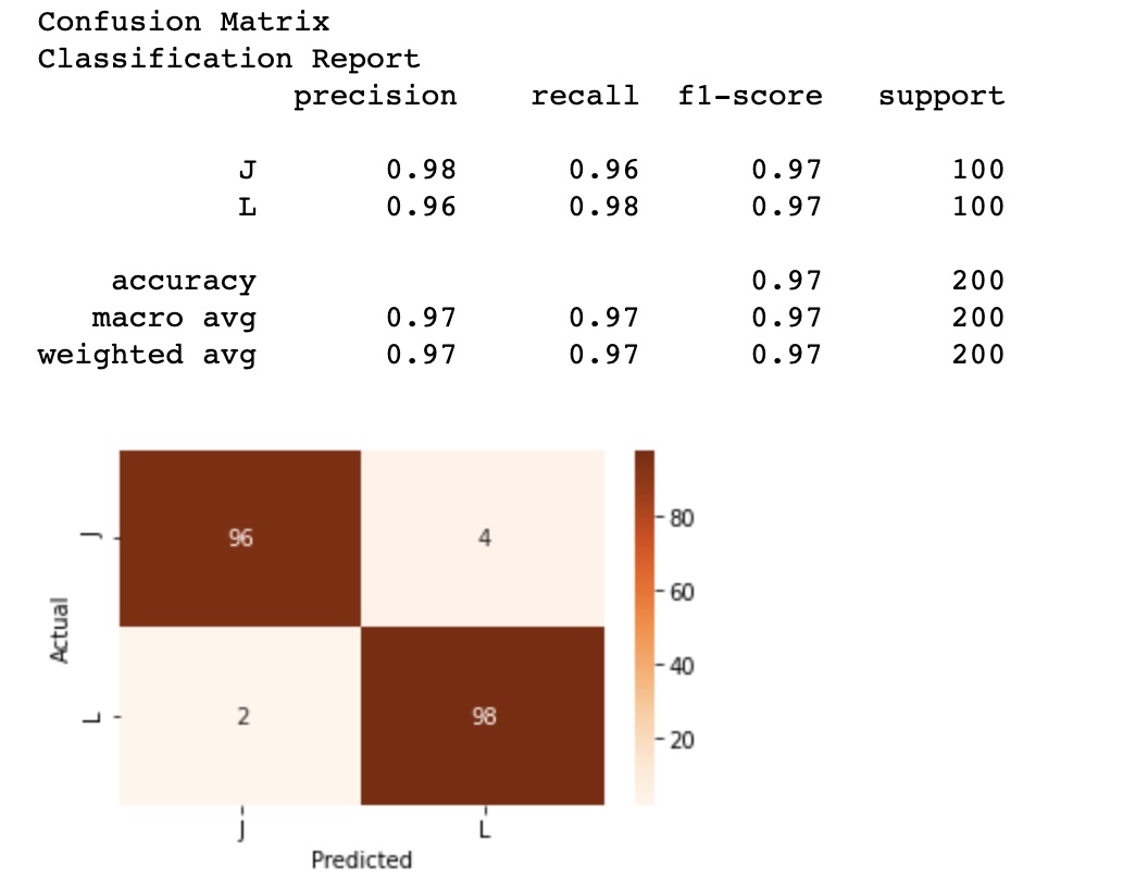
Accuracy is a key indicator but even with a 2-class classification problem, it is a common error to ignore more subtle information such as the confusion matrix. Using the following snippet and the scikit learn library. We are able to collect a full classification report along a confusion matrix. Again, here all signals are green, and we see the results of a very efficient classifier. Yet, let us not forget that the game has been tricked!
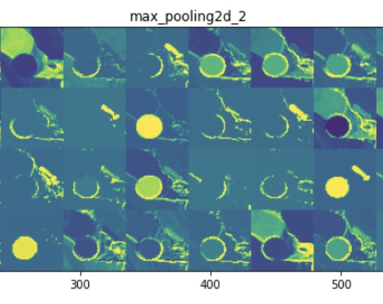
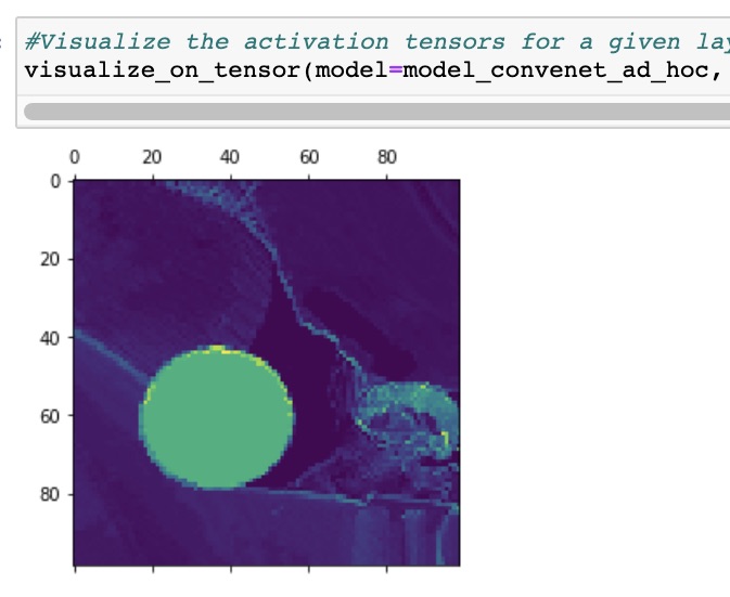
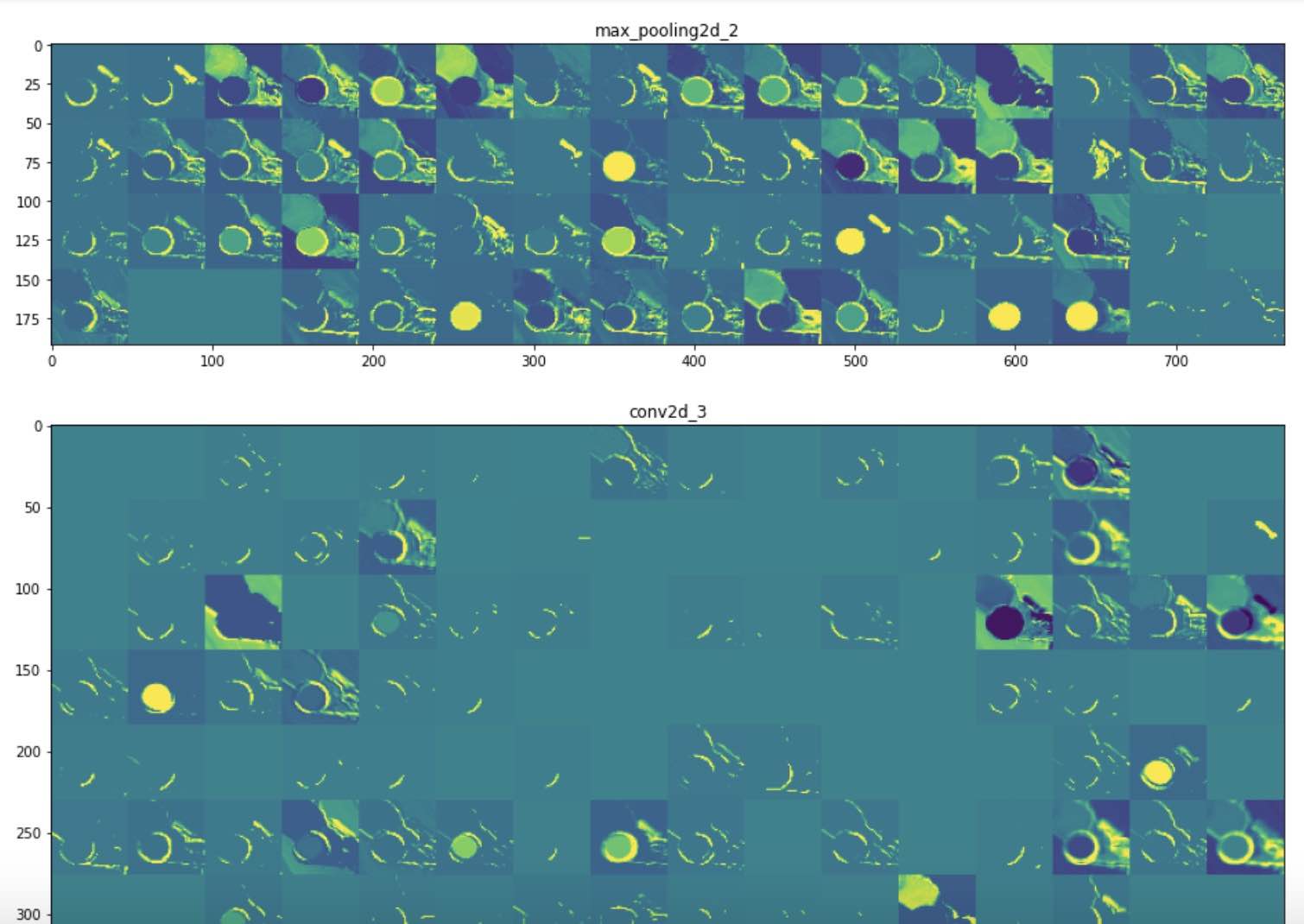
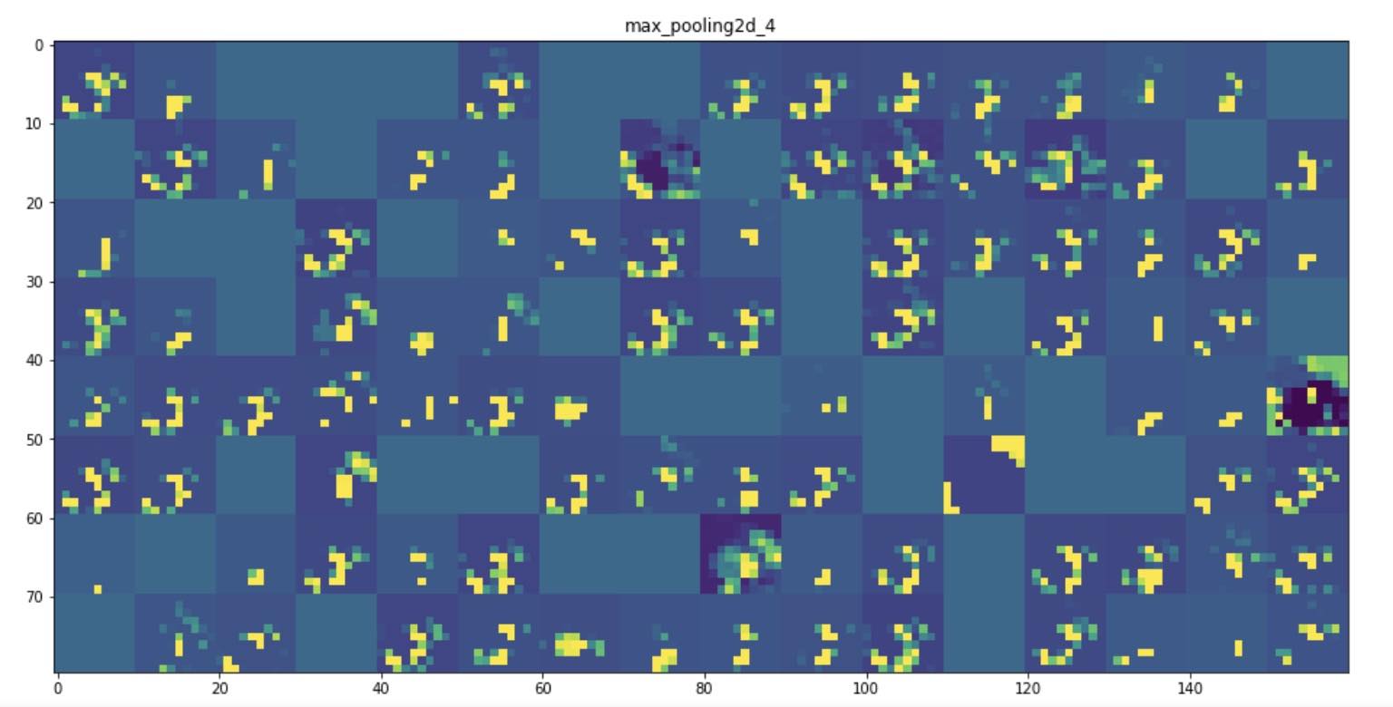
Going beyond and observe Conv2d learnings with an activation model
Again, we use a technique well exposed in the François Chollet’s book.
The idea is to build a multi output model based on the successive outputs of the base convolutional layers. Thanks to the successive ReLu layers, we can plot the activation maps from the outputs of these layers. The following visuals illustrate well that our Convnet base model has successfully learned the geometrical shape: the curved stroke of ellipses and the squared edges of rectangles.
Back to the real face recognition problem
Now it is time to get back to our original problem: classification of my baby girls without relying on any trick, just with face recognition on the original images. The simple Convnet in the previous section will not be sufficient to build a classifier with significant accuracy. We will need bigger artillery.
The experiments provided in this section can be found in this notebook.
Using the InceptionResNetV1 as a base model
InceptionResNetV1 is a deep learning model that has proven to be one of the state-of-the-art very deep architecture for convolutional networks. It also uses the concept Residual Neural Networks.
We use its implementation provided originally by Sefik Ilkin Serengil whom was also reusing parts of the implementation provided by David Sandberg.
For our classification problem, we use InceptionResNetV1 as the base (then very deep) network. On top of it we flatten the tensors and bring Dense and Dropout layers to serve as classification.
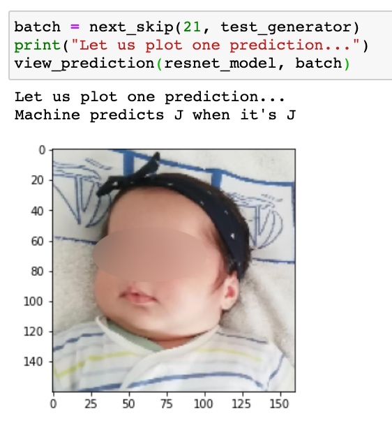
Achieving nearly 0.80 accuracy
We conducted some experiments when trying to make InceptionResNetV1 without any prior weights tuning, which means without using pre-trained experimentations (sometimes called Transfer Learning). Without any surprise, the model could not reach significant validation accuracy (i.e. significantly above 0.6 in accuracy). Our dataset, even with data augmentation, is too small to let a deep architecture “learn” what are the key elements that constitute the characteristics of a human face.
Therefore, we reuse pretrained weights from facenet database, provided by David Sandberg and Sefik Ilkin Serengil in his blog post.
Thanks to our GPU we were able to retrain the full model composed of a InceptionResNetV1 base with our top layers classifiers. We did not even have to recourse to fine-tuning techniques where the first layers weights need to be frozen.
After a dozen of minutes of training, I was happy to see the following training and validation accuracy curves.
This shows all the positive signs of a successfully trained ML algorithm. Therefore, let us examine the performance on the test dataset, i.e. the one that has not been fed to the algorithm before.
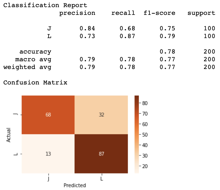
The classification reports and confusion matrix on the test dataset confirm the measure on the validation set. We achieve nearly 80% of accuracy. One interesting thing is, from the report, J. looks to be a little be more difficult for our model to classify than L. Honestly, I have no assumption on what could cause this. A deeper analysis by examining layers in the spirit of what has been presented above could be conducted.
Conclusion
I did not spend time trying to tune so much the InceptionResNetV1 hyperparameters. I tweaked a little the top layers of the classifier. No doubt that there is room for great improvements here. This can constitute a follow up blog post.
Also, I did not confront other algorithms and deeplearning architectures. I quickly gave a try to the Deepface Keras implementation but without significant results. I did not spend time investigating why this was not working. Once again this could be part of an interesting follow up. Ideally, I would also benchmark this DLib implementation.
By conducting these experiments, I confirm that it is nearly impossible to perform “real” recognition on faces without some kind of pretrained models if you have at hands this small amount of face data.
Finally, I learnt a lot. It is always a good thing to try things on your own data. This is how you learn to tackle real-life problems in datascience.